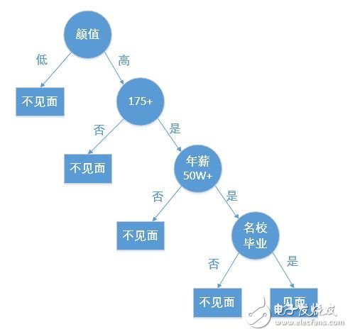
A decision tree is a fundamental classification and regression technique. This article primarily focuses on the decision tree used for classification. A decision tree is a tree-like structure that classifies data based on certain conditions. For example, the process of matching a female client on a high-end dating website can be represented as a decision tree:

Creating a decision tree from a given dataset is part of machine learning. While building a decision tree may take time, using it is fast and efficient. The most critical aspect in constructing a decision tree is determining which feature to use for classification. A good feature can maximize the separation of the dataset, bringing order to chaos.
The question then arises: how do we measure the level of disorder or order in a dataset? In information theory and probability statistics, entropy is used to quantify the uncertainty of a random variable, representing the degree of disorder.
Let’s consider a sample dataset D as an example throughout this article:
| Serial Number | Ankle | Survive |
|---------------|-------|---------|
| 1 | Yes | Yes |
| 2 | Yes | Yes |
| 3 | No | No |
| 4 | No | No |
| 5 | No | No |
The code to create this dataset is as follows:
```python
def create_data_set():
dataSet = [[1,1,'yes'],
[1,1,'yes'],
[1,0,'no'],
[0,1,'no'],
[0,1,'no']]
labels = ['no surfacing', 'flippers']
return dataSet, labels
```
---
### 2. Entropy, Information Gain, and Information Gain Ratio
#### 2.1 Entropy
The term "entropy" was first introduced to me in high school chemistry, where it was used to describe the degree of disorder in a system. Although the context differs, the concept remains similar in information theory — entropy measures the uncertainty or disorder in a random variable. The higher the entropy, the more chaotic the system.
In information theory, if X is a discrete random variable with a finite number of values and a probability distribution P(X), the entropy H(X) is defined as:
$$
H(X) = -\sum_{i=1}^{n} P(x_i) \log_2 P(x_i)
$$
To calculate entropy in Python, here's a function:
```python
import math
def cal_Ent(dataSet):
num = len(dataSet)
labels = {}
for row in dataSet:
label = row[-1]
if label not in labels.keys():
labels[label] = 0
labels[label] += 1
ent = 0.0
for key in labels:
prob = float(labels[key]) / num
ent -= prob * math.log(prob, 2)
return ent
```
#### 2.2 Information Gain
Information gain measures how much uncertainty about the class (Y) is reduced by knowing the value of a feature (X). It is calculated as the difference between the entropy before and after splitting the dataset based on a feature.
$$
\text{Information Gain} = H(Y) - H(Y|X)
$$
When estimating probabilities from data, these are referred to as empirical entropy and empirical conditional entropy.
To select the best feature for splitting, we compute the information gain for each feature. Here's how it's done:
```python
def split_data_set(dataSet, axis, value):
retDataSet = []
for row in dataSet:
if row[axis] == value:
reducedRow = row[:axis]
reducedRow.extend(row[axis+1:])
retDataSet.append(reducedRow)
return retDataSet
def choose_best_feature(dataSet):
numFeatures = len(dataSet[0]) - 1
baseEnt = cal_Ent(dataSet)
bestInfoGain = 0.0
bestFeature = -1
for i in range(numFeatures):
featList = [example[i] for example in dataSet]
uniqueVals = set(featList)
newEnt = 0.0
for value in uniqueVals:
subDataSet = split_data_set(dataSet, i, value)
prob = len(subDataSet) / float(len(dataSet))
newEnt += prob * cal_Ent(subDataSet)
infoGain = baseEnt - newEnt
if infoGain > bestInfoGain:
bestInfoGain = infoGain
bestFeature = i
return bestFeature
```
This method is used in the ID3 algorithm, which builds decision trees by selecting the feature with the highest information gain.
#### 2.3 Information Gain Ratio
While information gain is effective, it tends to favor features with many possible values. To address this, the information gain ratio is used. It adjusts the information gain by dividing it by the intrinsic value of the feature, which measures how evenly the feature splits the data.
$$
\text{Information Gain Ratio} = \frac{\text{Information Gain}}{\text{Intrinsic Value}}
$$
This helps in selecting more balanced features and avoids bias toward features with high cardinality.
Copper Clad Steel ,Copper Clad Steel Highly Conductive,Copper Clad Steel Strand,Anti-Oxidation Copper-Clad Stee
changzhou yuzisenhan electronic co.,ltd , https://www.ccs-yzsh.com