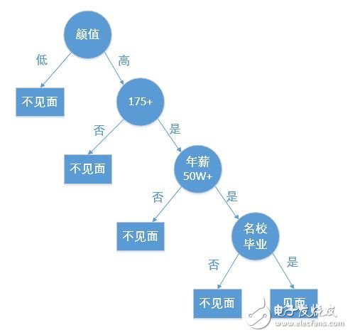
A decision tree is a fundamental method used for classification and regression. This article primarily focuses on the decision tree used for classification. A decision tree is a tree-like structure that classifies data based on certain conditions. For example, the process of matching a female client on a high-end dating website can be represented as a decision tree:

Creating a decision tree from a given dataset is a core topic in machine learning. While building a decision tree may take more time, using it for prediction is very fast. The most critical challenge when constructing a decision tree is determining which feature to use as the classification criterion. A well-chosen feature can maximize the separation of the dataset, transforming disorder into order.
But how do we measure the level of order in a dataset? In information theory and probability statistics, entropy is used to quantify the uncertainty of a random variable—essentially, the degree of disorder. The higher the entropy, the more uncertain or chaotic the data is.
Let’s consider a sample dataset D as an example throughout this article:
| No Surfacing | Flippers | Class |
|--------------|----------|-------|
| 1 | 1 | yes |
| 1 | 1 | yes |
| 1 | 0 | no |
| 0 | 1 | no |
| 0 | 1 | no |
The Python code to create this dataset is as follows:
```python
def create_data_set():
dataSet = [[1,1,'yes'],
[1,1,'yes'],
[1,0,'no'],
[0,1,'no'],
[0,1,'no']]
labels = ['no surfacing', 'flippers']
return dataSet, labels
```
---
### 2. Entropy, Information Gain, and Information Gain Ratio
#### 2.1 Entropy
The first time I encountered the term "entropy" was in my high school chemistry class, where it referred to the degree of disorder in a system. Though the context was different, the concept of entropy as a measure of chaos or uncertainty remains similar in both fields.
In information theory and probability, let X be a discrete random variable with a finite number of values and a probability distribution P(X). The entropy H(X) is defined as:
$$
H(X) = -\sum_{i=1}^{n} p(x_i) \log_2 p(x_i)
$$
Here's a Python function to calculate the entropy of a dataset, where the last element of each row represents the class label:
```python
import math
def calc_entropy(dataSet):
num_entries = len(dataSet)
labels = {}
for row in dataSet:
current_label = row[-1]
if current_label not in labels:
labels[current_label] = 0
labels[current_label] += 1
entropy = 0.0
for key in labels:
prob = float(labels[key]) / num_entries
entropy -= prob * math.log(prob, 2)
return entropy
```
#### 2.2 Information Gain
Information gain measures how much uncertainty (or entropy) is reduced by knowing the value of a particular feature. It is calculated as the difference between the entropy before and after splitting the dataset based on a feature.
$$
\text{Information Gain} = H(Y) - H(Y|X)
$$
Where $ H(Y) $ is the entropy of the class before the split, and $ H(Y|X) $ is the conditional entropy after the split.
To select the best feature for splitting, we calculate the information gain for each feature and choose the one with the highest value.
Here's a function to split the dataset based on a specific feature and its value:
```python
def split_data_set(dataSet, axis, value):
retDataSet = []
for row in dataSet:
if row[axis] == value:
reducedRow = row[:axis]
reducedRow.extend(row[axis+1:])
retDataSet.append(reducedRow)
return retDataSet
```
And here's a function to find the best feature to split on:
```python
def choose_best_feature(dataSet):
num_features = len(dataSet[0]) - 1
base_entropy = calc_entropy(dataSet)
best_info_gain = 0.0
best_feature = -1
for i in range(num_features):
feat_list = [example[i] for example in dataSet]
unique_vals = set(feat_list)
new_entropy = 0.0
for value in unique_vals:
sub_dataset = split_data_set(dataSet, i, value)
prob = len(sub_dataset) / float(len(dataSet))
new_entropy += prob * calc_entropy(sub_dataset)
info_gain = base_entropy - new_entropy
if info_gain > best_info_gain:
best_info_gain = info_gain
best_feature = i
return best_feature
```
The ID3 algorithm uses information gain to select the best feature for splitting during the construction of a decision tree.
#### 2.3 Information Gain Ratio
While information gain is effective, it tends to favor features with many possible values, which can lead to overfitting. To address this, the C4.5 algorithm introduces the **information gain ratio**, which normalizes the information gain by the intrinsic information of the feature.
$$
\text{Gain Ratio} = \frac{\text{Information Gain}}{\text{Intrinsic Value}}
$$
This helps in selecting features that are more balanced and less biased toward those with high cardinality.
Tinned Copper Clad Steel,Professional Tinned Copper Clad Steel,Heat-Resistant Tinned Copper-Clad Steel,Tinned Copper Clad Steel Metal Wire
changzhou yuzisenhan electronic co.,ltd , https://www.ccs-yzsh.com