Part of the experience and insights on how to "train" a neural network

The author begins with a simple mathematical definition of neural networks and further describes the basic optimization algorithms along with loss functions, activation functions, and backpropagation. After understanding these basics, this paper describes in detail the current very popular learning algorithms such as the momentum method. In addition, other important neural network training methods such as Adam and genetic algorithms will be introduced later in this series.

I. Introduction

This article is part of the author's experience and insights on how to "train" neural networks, and to deal with the basic concepts of neural networks. This article also describes gradient descent (GD) and some of its variants. In addition, the series will introduce the current popular learning algorithms in the following sections, such as:

Momentum Stochastic Gradient Descent Method (SGD)

RMSprop algorithm

Adam algorithm (adaptive moment estimation)

Genetic algorithm

The author begins with a very simple neural network introduction in the first part, simple enough to justify the concepts we are talking about. The author will explain what a loss function is and what it means to "train" a neural network or any other machine learning model. The author's explanation is not a comprehensive and in-depth introduction to neural networks. In fact, the author hopes that our readers have already understood these related concepts. If the reader wants to better understand how the neural network works, readers can read related books such as Deep Learning, or refer to the list of related learning resources provided at the end of the article.

The author explains everything in the cat and dog identification contest (https://) conducted on kaggle a few years ago. The task we face in this game is to give a picture and judge whether the animal in the picture is a cat or a dog.

II. Defining neural networks

The generation of artificial neural networks (ANN) is inspired by the working mechanism of the human brain. Although this simulation is not very strict, ANN does have several similarities with their biological creators. They consist of a certain number of neurons. So, let's take a look at a single neuron.

Single neuron

The next neuron we will talk about is a slightly different version of the simplest neuron called "perceptory" from Frank Rosenblatt in 1957. All the changes I made were for simplification, because I won't cover the in-depth explanation of neural networks in this article. I just tried to give the reader an intuitive understanding of how neural networks work.

What is a neuron? It's a mathematical function, with a certain amount of value as input (regardless of how much you want as input), the neuron I'm drawing above has two inputs. We record each input as x_k, where k is the index of the input. For each input x_k, the neuron assigns it another number w_k, and the vector consisting of these parameters w_k is called the weight vector. It is these weights that make each neuron unique. In the process of testing, the weights will not change, but in the process of training, we have to change these weights to "tune" our network. I will discuss this in a later article. As mentioned earlier, a neuron is a mathematical function. But what kind of function is it? It is a linear combination of weights and inputs, and some nonlinear function based on this combination. I will continue to explain further. Let's take a look at the first linear combination.

A linear combination of input and weight.

The above formula is the linear combination I mentioned. We want to multiply the input by the corresponding weight and then sum all the results. The result will be a number. The last part - is to apply some kind of nonlinear function to this number. The most commonly used nonlinear function today is a piecewise linear function called ReLU (rectified linear unit) with the following formula:

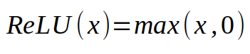
The expression of a linear rectification unit.

If our number is greater than 0, we will use this number. If it is less than 0, we will replace it with 0. This nonlinear function used on linear neurons is called an activation function. The reason we have to use some kind of nonlinear function will become apparent later. To summarize, neurons use a fixed number of inputs and (scalars) and output a scalar activation value. The neurons drawn above can be summarized into a formula as follows:

Put a little bit ahead of what I want to write. If we take the task of identifying dogs and cats as an example, we will use the image as a neuron input. Maybe you will wonder: how to pass a picture to a neuron when it is defined as a function. You should remember that the way we store the image in the computer is to represent it as an array, where each number represents the brightness of a pixel. So, the way to pass a picture to a neuron is to expand a 2-dimensional (or 3-dimensional color image) array to get a one-dimensional array, and then pass those numbers to the neurons. Unfortunately, this causes our neural network to depend on the size of the input image, and we can only process a fixed-size image defined by the neural network. Modern neural networks have found ways to solve this problem, but we are still designing neural networks under this limitation.

Now let's define the neural network. A neural network is also a mathematical function, which is a number of interconnected neurons. The connection here refers to the output of one neuron being used as input to another neuron. The picture below is a simple neural network, and I hope that this definition can be used to explain this definition more clearly.

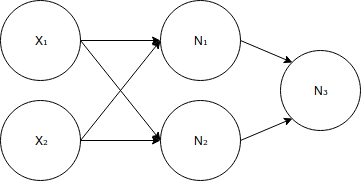
A simple neural network.

The neural network defined in the figure above has 5 neurons. As you can see, this neural network is made up of three fully connected layers, that is, each neuron in each layer is connected to each neuron in the next layer. How many layers of your neural network, how many neurons in each layer, and how the neurons are linked together, these factors together define a neural network architecture. The first layer is called the input layer and contains two neurons. This layer of neurons is not the neuron I mentioned before, in a sense, it does not perform any calculations. They here only represent the input of the neural network. The neural network's need for nonlinearity stems from two facts: 1) our neurons are connected together; 2) linear function-based functions are linear. So, if you don't apply a nonlinear function to each neuron, the neural network will be a linear function, then it is not more powerful than a single neuron. The last point to emphasize is that we usually want a neural network to have an output size between 0 and 1, so we will treat it as a probability. For example, in the case of cat and dog identification, we can treat the output close to 0 as a cat and the output close to 1 as a dog. To accomplish this, we will apply a different activation function on the last neuron. We will use the sigmoid activation function. With regard to this activation function, you only need to know that its return value is a number between 0 and 1, which is exactly what we want. After explaining this, we can define a neural network corresponding to the above figure.

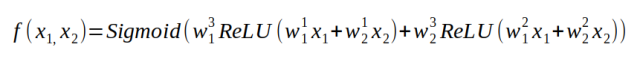
Define a function of a neural network. The superscript of w represents the index of the neuron, and the subscript represents the index of the input.

Finally, we get a function that takes a few numbers as input and outputs another number between 0 and 1. In fact, it doesn't matter how this function is expressed. What's important is that we parameterize a nonlinear function with some weights. We can change this nonlinear function by changing these weights.

III. Loss function

Before we begin to discuss the training of neural networks, the last thing we need to define is the loss function. The loss function is a function that tells us how well the neural network performs on a particular task. The most intuitive way to do this is to send a number along each neural network to each training sample, and then weigh the number with the actual number we want to get squared, so that the calculation is The distance between the predicted value and the true value, and the training neural network is expected to reduce this distance or loss function.

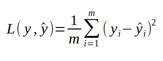
The y in the above equation represents the number we want to get from the neural network, the actual result of a sample that y hat refers to through the neural network, and i is the index of our training sample. We still take the identification of cats and dogs as an example. We have a dataset consisting of pictures of cats and dogs. If the picture is a dog, the corresponding label is 1. If the picture is a cat, the corresponding label is 0. This tag is the corresponding y, the result we want to get through the neural network when passing a picture to the neural network. To calculate the loss function, we must iterate through each picture in the dataset, calculate y for each sample, and then calculate the loss function as defined above. If the loss function is large, then our neural network performance is not very good, we want the loss function to be as small as possible. To gain a deeper understanding of the connection between the loss function and the neural network, we can rewrite this formula and replace y with the actual function of the network.

IV. Training

At the beginning of training the neural network, the weights are randomly initialized. Obviously, the initialized parameters will not give good results. In the process of training, we want to start with a very bad neural network and get a network with high accuracy. In addition, we also hope that the function value of the loss function becomes extremely small at the end of the training. It is possible to improve the network because we can change the function by adjusting the weight. We want to find a function that performs much better than the initialized model.

The problem is that the training process is equivalent to minimizing the loss function. Why is it to minimize losses rather than maximize them? The results prove that the loss is a function that is easier to optimize.

There are many algorithms for function optimization. These algorithms can be gradient-based or not gradient-based because they can use either the information provided by the function or the information provided by the function gradient. One of the simplest gradient-based algorithms is called Random Gradient Descent (SGD), which is the algorithm I will introduce in this article. Let's see how it works.

First, we need to remember what the derivative of a variable is. Let's take the simpler function f(x) = x as an example. If you remember the calculus rule you learned in high school, we know that this function has a derivative of 1 at each x. So what information can the derivative tell us? The derivative describes how fast the function value changes when we let the argument change infinitely small steps in the positive direction. It can be written in the following mathematical form:

What it means is that the amount of change in the function value (on the left side of the equation) is approximately equal to the product of the derivative of the function at a corresponding variable x and the increment of x. Going back to the simplest example we just mentioned, f(x) = x, where the derivative is everywhere, which means that if we change x by a small step ε in the positive direction, the change in the output of the function is equal to the product of 1 and ε. It is just ε itself. It is easier to check this rule. In fact this is not an approximation, it is accurate. why? Because our derivatives are the same for every x. But this does not apply to most functions. Let's look at a slightly more complicated function f(x) = x^2.

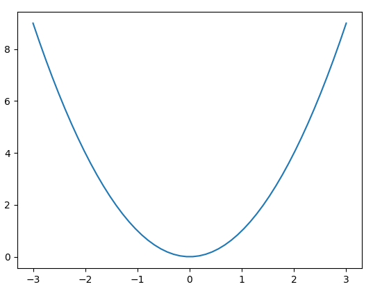
We can know from the knowledge of calculus that the derivative of this function is 2*x. Now if we move the ε of a step from a certain x, it is easy to see that the corresponding function increment is not exactly equal to the calculation in the above formula.

Gradient is now a vector of partial derivatives whose elements are the derivatives of some of the variables on which this function depends. For the simple function we are currently considering, this vector has only one element, because the function we use has only one input. For more complex functions (such as our loss function), the gradient will contain the derivative of each variable corresponding to the function.

In order to minimize a loss function, how can we use this information provided by the derivative? Still return to the function f(x) = x^2. Obviously, this function takes the minimum value at the point of x=0, but how does the computer know? Suppose we get a random initial value of x of 2, and the derivative of the function is equal to 4. This means that if x changes in the positive direction, the increment of the function will be four times the increment of x, so the function value will increase instead. Instead, we want to minimize our function, so we can change x in the opposite direction, which is the negative direction. To ensure that the function value is reduced, we only change a small step. But how much can we change in one step? Our derivatives only guarantee that the function value will decrease when x changes infinitely small in the negative direction. Therefore, we hope to use some hyperparameters to control how much can be changed at a time. These hyperparameters are called learning rates, which we will talk about later. Let's take a look now, what happens if we start at -2. The derivative here is -4, which means that if you change x in the positive direction, the value of the function will become smaller, which is exactly what we want.

Have you noticed the rules here? When x>0, our derivative value is also greater than 0, we need to change in the negative direction. When x<0, our derivative value is less than 0, we need to change in the positive direction, we always need to be toward the derivative. Change x in the opposite direction. Let us also quote the same idea for gradients. A gradient is a vector that points in a certain direction of space. In fact, it points to the direction in which the value of the function increases most sharply. Since we want to minimize our function, we will change the argument in the opposite direction to the gradient. Now apply this idea to us. In neural networks, we treat input x and output y as fixed numbers. The variable we want to derive is the weight w, because we can improve the neural network by changing these weight classes. If we calculate the gradient corresponding to the weight of the loss function and then change the weight in the opposite direction to the gradient, our loss function will also decrease until it converges to a local minimum. This algorithm is called gradient descent. The algorithm for updating weights in each iteration is as follows:

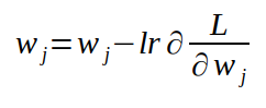
Each weight value is subtracted from the product of its corresponding derivative and learning rate.

Lr in the above equation represents the learning rate, which is the variable that controls the size of the step in each iteration. This is an important hyperparameter that we need to adjust when training neural networks. If the learning rate we choose is too large, it will cause the stepping to be too large, so that the minimum value is skipped, which means your algorithm will diverge. If the learning rate you choose is too small, it may take too much time to converge to a local minimum. People have developed some good techniques to find the best learning rate, but this content is beyond the scope of this article.

Unfortunately, we cannot apply this algorithm to train neural networks because of the formula for the loss function.

As you can see in my previous definition, the formula for our loss function is the average of the sum. From the principle of calculus we can know that the sum of the differentials is the differentiation of the sum. So, in order to calculate the gradient of the loss function, we need to iterate through each sample in our data set. It is very inefficient to perform a gradient drop in each iteration because each iteration of the algorithm only increases the loss function in a small step. To solve this problem, there is another small batch gradient descent algorithm. The algorithm's method of updating weights is constant, but we won't calculate exact gradients. Instead, we approximate the gradient on a small batch of datasets and then use this gradient to update the weights. Mini-batch does not guarantee that the weight will be changed in the best direction. In fact, it usually doesn't. When using the gradient descent algorithm, if the chosen learning rate is small enough, you can guarantee that your loss function will decrease in each iteration. But this is not the case when using Mini-batch. Your loss function will decrease over time, but it will fluctuate and will have more "noise".

The batch size used to estimate the gradient is another hyperparameter that you must choose. Usually, we want to choose as large a batch as we can handle. But I rarely see others using a batch size larger than 100.

The extreme case of mini-batch gradient descent is that the batch size is equal to 1, and this form of gradient descent is called stochastic gradient descent (SGD). Usually in many literatures, when people say that random gradients fall, they actually refer to mini-batch random gradients. Most deep learning frameworks let you choose the batch size for a random gradient drop.

The above is the basic concept of gradient descent and its variants. But more and more people are using more advanced algorithms recently, most of which are based on gradients. The authors will introduce these optimization methods in the next section.

VII. Back Propagation (BP)

The only thing left about gradient-based algorithms is how to calculate gradients. The quickest way is to analytically give the derivative of each neuron architecture. I think that when the gradient encounters a neural network, I should not say that this is a crazy idea. The very simple neural network we defined earlier is quite difficult, and it has only six parameters. The parameters of modern neural networks are millions.

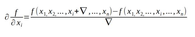
The second method is to use the following formula we learned from calculus to approximate the gradient. In fact, this is the easiest method.

Although this method is very easy to implement, it is very computationally intensive.

The last method of calculating the gradient is a compromise between analytical difficulty and computational cost. This method is called a reverse pass. Backpropagation is beyond the scope of this article. If you want to know more, check out the fifth section of Goodfellow's Deep Learning, Chapter 6, which provides a very detailed introduction to backpropagation algorithms.

VI. Why does it work?

When I first learned about neural networks and how it works, I understand all the equations, but I am not quite sure that they will work. This idea is a bit grotesque for me: use a few functions to find some derivatives, and eventually get a recognition of whether the picture is a cat or a dog. Why can't I give you a good intuition about why the neural network will work so well? Please note the following two aspects.

1. The problems we want to solve with neural networks must be expressed in mathematical form. For example, for the identification of dogs and cats: we need to find a function that takes all the pixels in a picture as input and then outputs the probability that the content in the picture is a dog. You can use this method to define any classification problem.

2. It may not be very clear why there is a function that separates the cat from the dog from a picture. The idea here is that as long as you have some datasets with inputs and labels, there will always be a function that performs well on a given dataset. The problem is that this function can be quite complicated. At this time, the neural network can help. There is a "universal approximation theorem", which means that a neural network with a hidden layer can approximate any function you want. How good you want it to be, how good it can be.

Momentum stochastic gradient descent algorithm

- This is the second part of a series on training neural network and machine learning model optimization algorithms. The first part is about random gradient descent. In this section, it is assumed that the reader has a basic understanding of neural networks and gradient descent algorithms. If the reader is ignorant of the neural network, or does not know how the neural network is trained, read the first part before reading this section.

In this section, in addition to the classic SGD algorithm, we also discuss the momentum method, which is generally better and faster than the random gradient descent algorithm. The momentum method [1] or the momentum SGD is a method that helps to accelerate the vector's gradient toward the correct direction, making it faster to converge. This is one of the most popular optimization algorithms, and many of the most advanced models are trained in this way. Before we talk about advanced algorithm-related equations, let's look at some basic mathematics about momentum.

Exponential weighted average

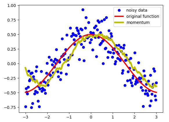
An exponentially weighted average is used to process the sequence of numbers. Suppose we have some noisy sequence S. In this example, I plotted the cosine function and added some Gaussian noise. As shown below:

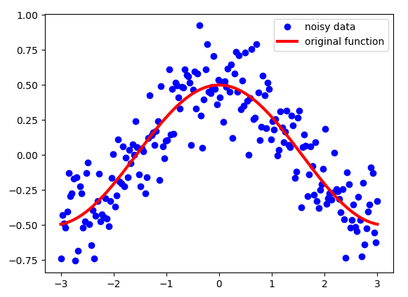
Note that although these points look very close, their x coordinates are different. That is, for each point, its x coordinate is a unique identifier, so this is also the index that defines each point in the sequence S.

We need to process this data instead of using them directly. We need some kind of "moving" average, which will "de-noise" the data to bring it closer to the original function. An exponentially weighted average can produce an image like this:

Momentum - data from an exponentially weighted average

As we have seen, this is a pretty good result. We get a smoother curve than the noisy data, which means we get closer to the original function than the initial data. The exponentially weighted average defines the new sequence V using the following formula:

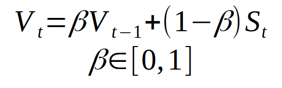
The sequence V is the yellow part of the scatter plot above. Beta is another hyperparameter with a value from 0 to 1. In the above example, take Beta = 0.9. 0.9 is a good value and is often used for SGD methods with momentum. We can intuitively understand Beta: we approximate the 1 / (1- beta) points after the sequence. Let's see how the beta selection affects the new sequence V.

Exponentially weighted average results when Beta values ​​are different.

As we can see, the smaller the Beta value, the greater the fluctuation of the sequence V. Because we have fewer average examples, the results are more "close" to the noise data. The larger the Beta value, such as when Beta = 0.98, the curve we get will be more rounded, but the curve is a bit offset to the right because the range we take the average becomes larger (beta = 0.98) 50). At Beta = 0.9, a good balance is achieved between these two extremes.

Mathematical part

This section is not necessary for your use of momentum in your project, so you can skip it. But this part explains more intuitively how momentum works.

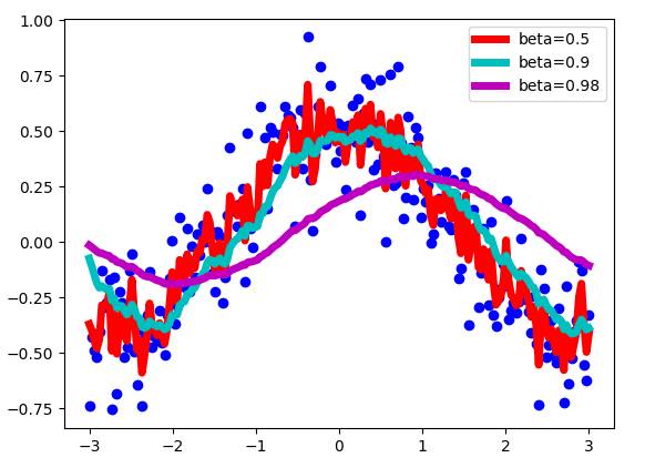
Let us extend the definition of three consecutive elements of the exponentially weighted average new sequence V.

V - new sequence. S - the original sequence.

Combine them and we can get:

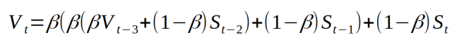
Simplify it and get:

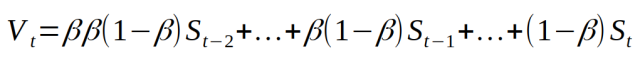
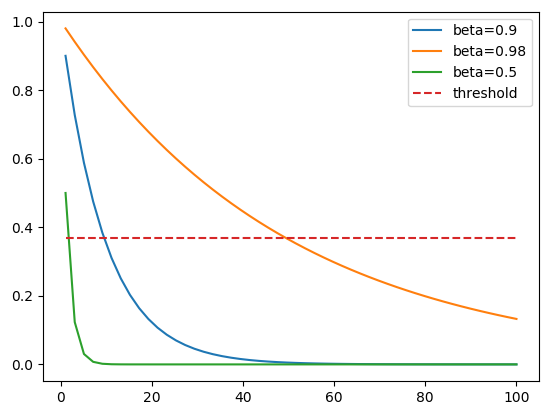
As can be seen from this equation, the Tth value of the new sequence depends on all previous values ​​1...t of the original sequence S. All values ​​from S are given a certain weight. This weight is the weight obtained by multiplying the (ti)th value of the sequence S by (1-beta). Because Beta is less than 1, when we take a beta on a power of a positive number, the value gets smaller. Therefore, the original value of the sequence S has a much smaller weight, and therefore the sequence S has less influence on the dot product produced by the sequence V. In some ways, the weight is so small that we can almost say that we "forget" this value because its impact is too small to be noticed. The advantage of using this approximation is that when the weight is less than 1 / e, a larger beta value will require more weights less than 1 / e. This is why the larger the beta value, the more we want to average the dot product. The chart below shows the speed at which the weight becomes smaller as the initial value of the sequence S changes compared to threshold = 1 / e. Here we "forget" the initial value.

The last thing to note is that the average value obtained for the first iteration will be poor because we don't have enough values ​​to average. We can solve this problem by using the bias revision of sequence V instead of using sequence V directly.

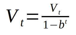
Where b = beta. When the value of t becomes large, the power of t of b cannot be distinguished from zero, so the V value is not changed. But when the value of t is small, this equation will produce better results. But because of the momentum, the machine learning process is very stable, so people are often too lazy to apply this part.

Momentum SGD method

We have defined a way to get the "moving" average of some sequences, which will change with the data. How do we apply it to the training of neural networks? It can average our gradients. I will explain below how this is done in Momentum and will continue to explain why it might get better results.

I will provide two definitions to define a SGD method with momentum, which is almost the same way to express the same equation in two different ways. First, it is Wu Enda's definition in the curriculum of Coursera Deep Learning Specialization (https://). The way he explains is that we define a momentum, which is the moving average of our gradient. Then we use it to update the weight of the network. As follows:

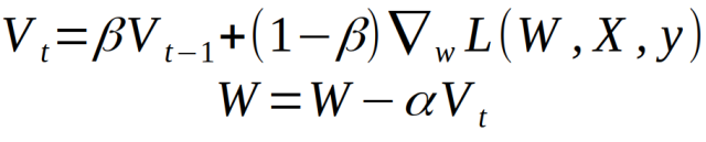
Where L is the loss function, the triangle symbol is the gradient wrt weight, and α is the learning rate. Another popular way to express momentum update rules is not so intuitive, except that the (1 - beta) term is omitted.

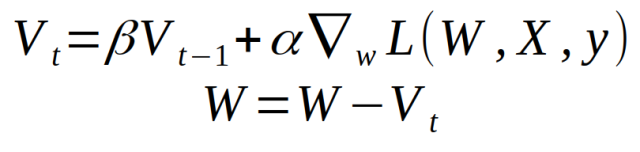
This is very similar to the first set of equations, the only difference being that the (1 - β) term needs to be adjusted to adjust the learning rate.

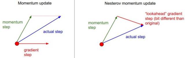
Nesterov accelerates the gradient

Nesterov Momentum is a slightly different version of the momentum update that has recently become more popular. In this version, you first get a point pointed to by the current momentum, and then calculate the gradient from this point. As shown below:

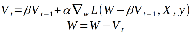
Nesterov momentum can be defined by:

Momentum working principle

Here I will explain why in most cases the momentum method is better than the classic SGD method.

Using the stochastic gradient descent method, we do not calculate the exact derivative of the loss function. Instead, we estimate a small batch of data. This means that we are not always moving in the best direction, because the result we get is "noisy." As I have listed in the chart above. Therefore, the weighted average of the indices can provide a better estimate that is closer to the derivative of the actual value than the result obtained by the noisy calculation. This is one of the reasons why momentum law may be better than traditional SGD.

Another reason is the ravine. A valley is an area in which a curve is steeper in one dimension than the other. In deep learning, the valley area can be approximated as the local minimum point, and this feature cannot be obtained by the SGD method. SGD tends to oscillate on narrow valleys because the negative gradient will descend along the steep side rather than along the valley to the best. Momentum helps accelerate the gradient in the right direction. As shown below:

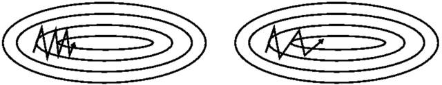
Left image - SGD without momentum, right image - SGD with momentum

in conclusion

I hope this section will provide some ideas on how the SGD method with momentum works and why it is useful. In fact, it is one of the most popular optimization algorithms for deep learning, which is often used more frequently than more advanced algorithms.